First we’ll get started with a standalone tracking “Job Option”, which will allow us to test out and configure some changes a little easier. This is distinct from the centrally produced and validated reco_tf, which is the widely-used way to run tracking (along with all of the other parts of ATLAS reconstruction!) and is shown a bit later in this tutorial. The general principle is the same, however!
Log in to lxplus and make a clean directory to work in.
ssh user@lxplus.cern.ch
mkdir funWithTracking && cd funWithTracking
Set up your environment and clone the tutorial repo.  If you’re not set up for Gitlab, please see the Gitlab tutorial in the main menu above!
setupATLAS
lsetup git python
git clone -b ssh://git@gitlab.cern.ch:7999/Atlas-Inner-Tracking/trackingworkshophandson.git
asetup Athena 22.0.40
mkdir run && cd run
The repo is full of example files we’ll explore in our tracking journey. You will find inside some example job options for running an example track reconstruction job on an RDO (simulated RAW data) file.
trackReconstructionExampleOptions.py
If you open this file in your browser of choice, you’ll see a variety of options that you can change to see the effect. For example:
# --- number of events to process
athenaCommonFlags.EvtMax     =  3
athenaCommonFlags.SkipEvents =   0
Now copy the job option to your run directory and execute simply by doing
cp ../trackingworkshophandson/trackReconstructionExampleOptions.py .
athena.py trackReconstructionExampleOptions.py
This will take a few minutes to run, so get a cup of coffee while you’re waiting. When you come back, you will find that this produces AOD.pool.root and ESD.pool.root, both of which can (at least partly) be opened and browsed with ROOT (look for the CollectionTree).
Next we want to make a few standard performance plots. The InDetPhysValMonitoring package features a comprehensive and configurable selection of histograms and plots, allowing many key tracking metrics (efficiencies, resolutions, number of hits/holes on tracks etc) to be accessed. We can run this as a separate step on your existing output files through Athena as follows:
athena --filesInput=AOD.pool.root InDetPhysValMonitoring/InDetPhysValMonitoring_topOptions.py
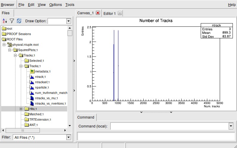
You should see a file M_output.root. If you open this in the TBrowser you should see a few directories, like this:
Contained within the folders are some varying plots about reconstructed tracks,vertices, and more. In the next subsections we’ll make a few example changes to the job option and see some effects!
