Validation Workflow -- Quick Plotting Setup for Local Checks (IDPhysValPlotting and More)

So you’re interested in comparing results from two different versions of tracking, or someone has asked you to make a comparison (lucky you! :-) ). This occurs relatively often – we might want to do this, for example, to see if there are any unintended effects for tracking in a new release or bug fix, or compare tests (with changes made by you or someone else) to get to the bottom of a previously observed difference. Depending on the type of check we are performing, we can use several tools. One is DCube, detailed in the previous section, while the other is a small package IDPhysValPlotting. Whichever one you want to use, there is a standardized workflow to perform these validation checks that is similar to the quick check earlier in the tutorial where we observed the effect on the InDetPhysValMonitoring distributions when changing the cut level.

Let’s say we have two different samples, tests, or releases we would like to compare. If you are producing these yourself, you will need to run reco_tf.py on an appropriate number of events as described in previous sections. For example, for the “q431” test (make sure your environment is set up with the version of Athena you are trying to run the test with!) we would do

Reco_tf.py --AMI=q431 --maxEvent 100

If you are starting with pre-produced AODs, we just need to run InDetPhysValMonitoring, preferably with the doExpertPlots flag for more in-depth inspection. Note that you do not have to run IDPVM with the same release that your AOD was produced with, you will likely want to run a recent release (or main) to get the most up to date assembly of plots. Which command you use depends on the version you are, using, however, like so:

runIDPVM.py --filesInput /path/to/your/input/file/ --doExpertPlots  --outputFile ./Test.root    ##RELEASE 22.0.45 AND NEWER
athena InDetPhysValMonitoring/InDetPhysValMonitoring_topOptions.py --filesInput /path/to/your/input/file/ - --doExpertPlots --outputFile ./Test.root ##RELEASE 22.0.44 AND OLDER

If you need to run a full sample (not recommended for quick checks) click here

you should have an output file with histograms, either the default M_output.root or whatever you specified as the output file name. If you are running local checks you will likely want to run more than a single file, e.g one lumiblock (generally ~5-10 files) so make sure to hadd these together:

hadd idpvm_testfile.root lbxxx_1.root lbxxx_2.root lbxxx_3.root

Now that you have IDPVM histograms for two different releases/tests of tracking you can either proceed with the DCube plotting procedure (detailed in the previous section) or use IDPhysValPlotting, a small package (link on gitlab here) designed to display IDPVM plots attractively. To use this you will need do some postprocessing on your combined output

postProcessIDPVMHistos idpvm_testfile.root

Make a new directory (outside of your main tutorial directory) and set up the IDPhysValPlotting package

mkdir physvalplotting/
cd physvalplotting
mkdir source; cd source/; 
git clone --recursive https://:@gitlab.cern.ch:8443/Atlas-Inner-Tracking/IDPhysValPlotting.git IDPhysValPlotting
cp IDPhysValPlotting/CMakeLists.forTopLevel.txt ./CMakeLists.txt
cd ..
mkdir build; cd build
asetup Athena,main,latest 
cmake ../source 
make
source x86_64-centos7-gcc11-opt/setup.sh
cd ..

The main program used for plotting is util/StandardPhysValComparison.cxx. It will auto-discover most interesting plots in the IDPVM output and plot them all into a (large) multi page PDF as well as individual PDF files. Histogram ranges etc are autodetected and ratios are also auto-computed. The block to edit in day-to-day work is lines ~37-45 _{^{(exact line numbers subject to change, depending on if changes are made between updates to this tutorial page!)}}, where we set the files to compare:

    std::vector<PlotFormat> formats{ 
        PlotFormat().Color(colRef).MarkerStyle(kFullSquare).LegendOption("PL").LegendTitle("Nominal detector").ExtraDrawOpts("LP").LineWidth(2)
        .CustomString("FileName","/eos/user/g/goblirsc/Tracking/PhysValPlottingExampleFiles/SglMu_master_nominal.IDPVM.root"),  // here you can set the file to load!
        
        PlotFormat().Color(colTest1).MarkerStyle(kFullDotLarge).LegendOption("PL").LegendTitle("No B-layer").ExtraDrawOpts("LP").LineWidth(2)
        .CustomString("FileName","/eos/user/g/goblirsc/Tracking/PhysValPlottingExampleFiles/SglMu_master_nominal.IDPVM.root"), // here you can set the file to load!
	  //PlotFormat().Color(colTest1).MarkerStyle(kFullDotLarge).LegendOption("PL").LegendTitle("No B-layer").ExtraDrawOpts("LP").LineWidth(2)
	  //.CustomString("FileName","/eos/user/g/goblirsc/Tracking/PhysValPlottingExampleFiles/SglMu_master_noBL.IDPVM.root"), // here you can set the file to load!
    }; 

Here you can change the files, plot color schemes, marker styles, labels, etc. Note that the vector can contain an arbitrary number of entries, so you are not limited to comparing just two setups at a time. The first element is considered the “reference”, and ratios are automatically prepared comparing each other setup to the reference.

Then you can just run the executable, making sure to recompile after making your changes!

cd build
make
source x86_64-centos7-gcc8-opt/setup.sh && cd ..
StandardPhysValComparison

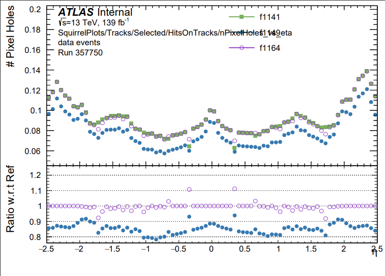
Then if you examine the resulting pdf output file you should see a (large) series of comparison plots like this:

StandardPhysValComparison example output

×

As an explicit check you can try performing these steps with the “default” and “alignment override” samples from the previous sections of the tutorial!