Overview of the ntuple content

Now that we have finished with the ntuple production steps, we will shift focus to doing some common analysis procedures on ntuples. The next few sections will focus on building an analysis from ntuples, but first let’s look at the ntuples that you have produced and the centrally-produced ntuples that you will use in the next steps.

Locally-produced ntuples

In the AnaAlgorithm steps up to this point, you have been running over a single ttbar sample and have added a small number of branches that hold information about a few physics object collections as well as missing transverse energy.

You can check the ntuple content by opening (from the run directory) submitDir/data-ANALYSIS/dataset.root and using a TBrowser:

root -l submitDir/data-ANALYSIS/dataset.root

(where -l disables the splash screen that can take some time to load), followed by simply:

TBrowser tb

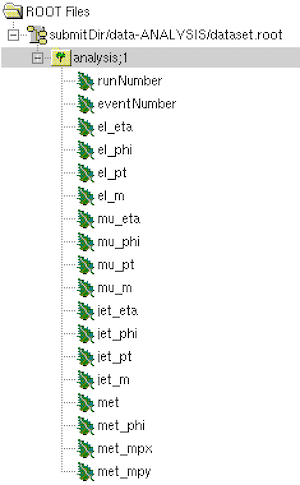
on the ROOT command line. The analysis tree should have the following branches:

As a reminder, the el_*, mu_* and jet_* branches are vectors of float corresponding to physics objects in each event while the met_* branches are float and runNumber and eventNumber are int since one value exists for each event. You can double click on any branch name to have ROOT draw it as a histogram.

Ntuples for analysis

A single simulated ttbar background sample is not sufficient to perform a physics analysis, and the set of information contained in your ntuple is very limited. Rather than having you extend the ntuple content and go through the time consuming step of running your code over several dozen samples, complete ntuples produced from the necessary samples are provided.

The full set of provided ntuples are available at /eos/user/j/jveatch/tutorial/ntuple/. The available samples are split into the following directories:

• signal: numerous leptoquark signal samples with varying masses, widths, and other model parameters
• data: a subset of the available ATLAS Run 2 detector data
• ttbar, wjets, etc.: the complete set of each background process that is important for the analysis

Within each directory, you will see files named *_out.root. For the signal and background samples, the six digit number in the file name corresponds to the sample’s DSID since these are all simulation. For the data samples, the number corresponds to the run number in which the data was collected.

Now let’s look at the content of one of the simulated samples using a TBrowser:

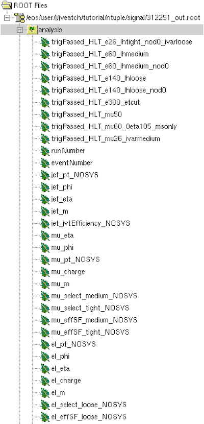
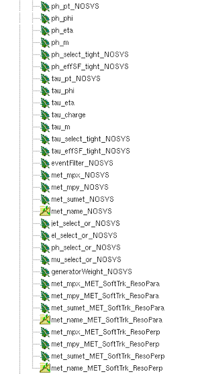
You will see almost all of the same branches that are in your locally-produced ntuple as well as a large number of additional branches.

In addition to the electron (el), muon (mu), and jet (jet) object branches, you also see branches for tau leptons (tau) and photons (ph). You also see additional met branches as well as branches holding information about trigger decisions.

Note that the ntuples contain tau and photon information even though they are not used in the analysis. This is generally considered bad practice because it adds size to the ntuples needlessly. Additionally, the inclusion of unneeded objects can impact the overlap removal procedure in a way that is not optimal for the analysis.

In this version of the ntuple, the met branches are vectors of floats, but this is not strictly necessary.

There are also several branches that end with NOSYS, which indicates that these represent nominal values without any systematic variations considered. More details about storing systematic variations will be presented in the systematic uncertainties section.

Furthermore, most physics object collections contain select and effSF branches. The former indicates whether each object in the collection passes the selection criteria of a working point and overlap removal for a particular systematic variation (nominal in this case). Only objects that pass at least one systematic variations are kept, those failing all available variations are discarded. The latter is a scale factor that needs to be applied on an object basis to correct for differences between simulation and detector data.

Finally, the generatorWeight branch includes weights that need to be applied to each simulated event to account for NLO contributions as well as scaling the simulation to the expected yields in data.

The data samples do not contain any scale factor or weight branches.